Learning notes about CG algorithm.

Conjugate Gradient Method: Principle

1. Motivation

The Conjugate Gradient (CG) method solves the linear system:

\[Ax = b.\]

where $A \in \mathbb{R}^{n \times n}$ is symmetric positive definite (SPD).

Equivalently, it minimizes the quadratic function:

\[f(x) = \frac{1}{2}x^T A x - b^T x.\]

Then let’s denote $\nabla f(x) = Ax - b = -r(x)$, where $r(x) = b - Ax$ is the residual.

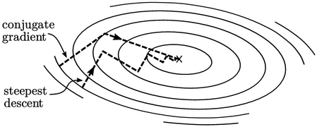
To solve this, one may suggest steepest descent moving along the negative gradient. But this often zigzags and converges slowly when $A$ is ill-conditioned. CG fixes this by choosing conjugate directions instead of just the current gradient.

2. Core Defination: Conjugacy

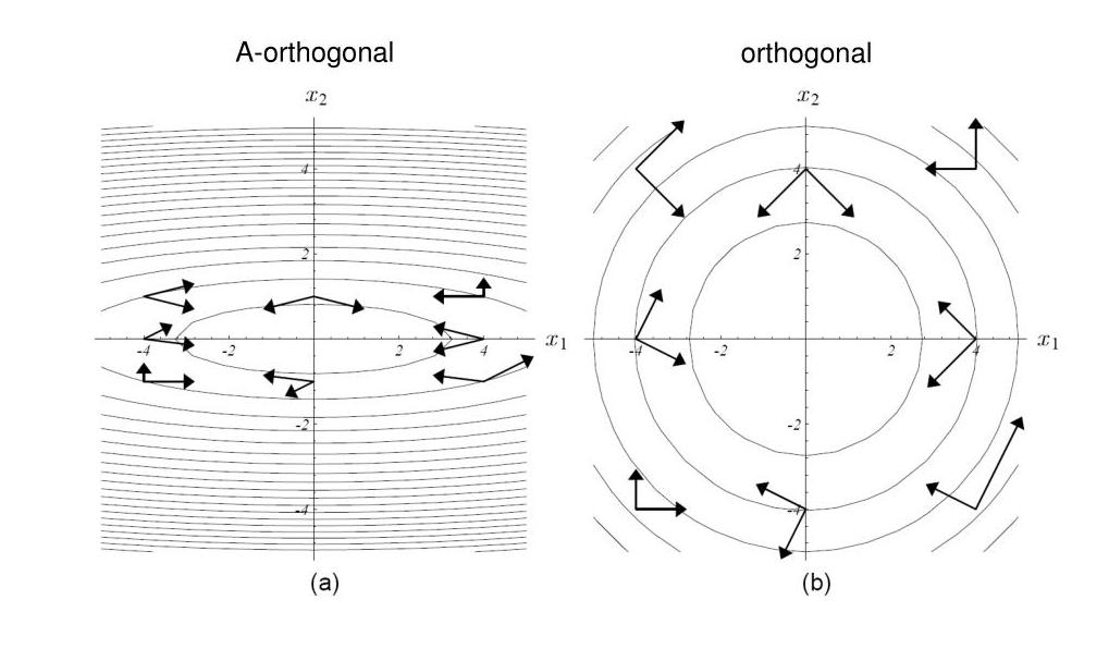
Two nonzero vectors $d_i$ and $d_j$ are conjugate (or $A$-orthogonal) if:

\[d_i^T A d_j = 0.\]

Why does this matter? Because if you minimize $f(x)$ along a direction $d_i$, and then later move along a conjugate direction $d_j$, you will not destroy the progress you made along $d_i$. The benefit you gained in the $d_i$-direction stays intact.

In CG, we build a set of search directions ${d_0, d_1, \dots, d_{n-1}}$ that are mutually conjugate. This ensures that moving along one direction does not spoil the optimality already achieved along previous directions.

3. Algorithm Structure

Initialization:

1. Set $x_{0}$
2. Compute residual: $r_{0} = b - A x_{0}$
3. Set first direction: $d_{0} = r_{0}$

At iteration $k$:

1. Compute step size $\alpha_k$
2. Update solution: $x_{k+1} = x_k + \alpha_k d_k$
3. Update residual: $r_{k+1} = r_k - \alpha_k A d_k$
4. Compute new conjugate direction: $d_{k+1} = r_{k+1} + \beta_k d_k$

3.1 Derivation of $\alpha_k$ (Step Size along Conjugate Direction)

We want to minimize $f(x_k + \alpha d_k)$ along direction $d_k$.

Substitute $x = x_k + \alpha d_k$ into $f(x)$:

\[f = \frac{1}{2}(x_k + \alpha d_k)^T A (x_k + \alpha d_k) - b^T (x_k + \alpha d_k).\]

Expanding and keeping only $\alpha$-dependent terms:

\[f = \text{const} + \alpha d_k^T (A x_k - b) + \frac{1}{2} \alpha^2 d_k^T A d_k.\]

Since $A x_k - b = -r_k$,

\[f = \text{const} - \alpha d_k^T r_k + \frac{1}{2} \alpha^2 d_k^T A d_k.\]

Set derivative to zero:

\[\frac{df}{d\alpha} = -d_k^T r_k + \alpha d_k^T A d_k = 0.\]

Hence:

\[\alpha_k = \frac{d_k^T r_k}{d_k^T A d_k}\]

Recall that $d_{k} = r_{k} + \beta_{k-1} d_{k-1}$, so we have

\[d_k^Tr_k = r_k^T r_k + \beta_{k-1} d_{k-1}^T r_k.\]

And $d_{k-1}^T r_k = 0$ since $x_k$ minimizes $f(x)$ along direction $d_{k-1}$:

\[∇f(x_k)^T d_{k-1} = -r_k^T d_{k-1} = 0.\]

So we can eventually write

\[\boxed{\alpha_k = \frac{r_k^T r_k}{d_k^T A d_k}}.\]

---

3.2 Constructing the Next Direction $d_{k+1}$

• Intuition

  Given a set of existing conjugate directions ${d_0, \dots, d_k}$, we want a new direction $d_{k+1}$ that is conjugate to all of them.

  A natural idea: start with the current residual $r_{k+1}$, then subtract all its “components” along the old conjugate directions:

\[\begin{aligned} d_{k+1} &= r_{k+1} + \sum_{j=0}^{k} \beta_j d_j, \\ \text{s.t.} \quad & d_{k+1}^T A d_i = 0, \quad i = 0, \ldots, k \end{aligned}\]

• Simplification

  By pluging $d_{k+1} = r_{k+1} + \sum_{j=0}^{k} \beta_j d_j$ into the conjugate requirements above, the target becomes solving:

  \[[r_{k+1} + \sum_{j=0}^{k}\beta_j d_j]^T A d_i = 0, \quad i = 0, \ldots, k,\] \[\text{i. e. } r_{k+1}^T A d_i + \sum_{i=0}^{k}\beta_j d_j^T A d_i, \quad i = 0, \ldots, k.\]

  Different directions are mutually conjugate, so we can elliminate lots of cross terms, leaving:

  \[r_{k+1}^T A d_i + \beta_i d_i^T A d_i = 0, \quad i = 0, \ldots, k.\]

• Site Property 2

  According to Property 2 (see next section for proof), we have $r_{k+1}^T A d_i = 0 $ for $ i \le k-1$, this core property hence simplifies our problem and the result gives:

  \[\beta_j = 0, \quad j = 0, \ldots, k-1,\] \[\beta_k = - \frac{r_{k+1}^T A d_k}{d_k^T A d_k}\]

• Simplify the Numerator

  From $r_{k+1} = r_k - \alpha_k A d_k$:

  \[A d_k = \frac{1}{\alpha_k} (r_k - r_{k+1})\]

  So:

  \[r_{k+1}^T A d_k = \frac{1}{\alpha_k} (r_{k+1}^T r_k - r_{k+1}^T r_{k+1})\]

  By Property 1 (see next section for proof), $r_{k+1}^T r_k = 0$. Hence:

  \[r_{k+1}^T A d_k = -\frac{r_{k+1}^T r_{k+1}}{\alpha_k}\]

• Simplify the Denominator

  From the definition of $\alpha_k$:

  \[\alpha_k = \frac{r_k^T r_k}{d_k^T A d_k}\]

  Thus:

  \[d_k^T A d_k = \frac{r_k^T r_k}{\alpha_k}\]

• Final Form

  \[\beta_k = -\frac{-\frac{r_{k+1}^T r_{k+1}}{\alpha_k}}{\frac{r_k^T r_k}{\alpha_k}} = \frac{r_{k+1}^T r_{k+1}}{r_k^T r_k}\]

  Therefore:

  \[\boxed{\beta_k = \frac{r_{k+1}^T r_{k+1}}{r_k^T r_k}}\]

  This is the Fletcher–Reeves formula.

  And the direction update simplifies to:

  \[\boxed{d_{k+1} = r_{k+1} + \beta_k d_k}\]

4. Two Key Properties

Property 1: Residuals are mutually orthogonal

For $i \neq j$:

\[r_i^T r_j = 0\]

Proof:

• At step $k$, $x_k$ is the minimizer along $d_{k-1}$, so $\nabla f(x_k)^T d_{k-1} = 0$, i.e. $r_k^T d_{k-1} = 0$.
• By induction, $r_k^T d_j = 0$ for all $j < k$.
• Since $d_j = r_j + \beta_{j-1} d_{j-1}$:

\[r_k^T r_j = r_k^T (d_j - \beta_{j-1} d_{j-1}) = 0 - 0 = 0\]

---

Property 2: $r_{k+1}^T A d_i = 0$ for all $i \le k-1$

This means that when constructing $d_{k+1}$, only the last old direction $d_k$ matters.

Proof:

From the residual update:

\[A d_i = \frac{1}{\alpha_i} (r_i - r_{i+1})\]

Thus for $i \le k-1$:

\[r_{k+1}^T A d_i = \frac{1}{\alpha_i} (r_{k+1}^T r_i - r_{k+1}^T r_{i+1}) = 0\]

by Property 1 (orthogonality of residuals).

5. Summary of the Algorithm

Initialize: $x_0$, $r_0 = b - A x_0$, $d_0 = r_0$
For $k = 1, 2, \dots$ until $r_k = 0$:
  $\alpha_k = \frac{r_k^T r_k}{d_k^T A d_k}$
  $x_{k+1} = x_k + \alpha_k d_k$
  $r_{k+1} = r_k - \alpha_k A d_k$
  $\beta_k = \frac{r_{k+1}^T r_{k+1}}{r_k^T r_k}$
  $d_{k+1} = r_{k+1} + \beta_k d_k$

6. Elegence

In exact arithmetic, CG converges to the exact solution $x^* = A^{-1}b$ in at most $n$ iterations.

This is because in $\mathbb{R}^n$, there can be at most $n$ mutually conjugate (hence linearly independent) directions.

Under the ridge setting, the story gets even more interesting.

In ridge regression, we solve:

\[(X^T X + \lambda I) w = X^T y\]

where $X \in \mathbb{R}^{N \times p}$ is the design matrix. This is exactly a linear system $A w = b$ with:

\[A = X^T X + \lambda I, \quad b = X^T y\]

The key insight: CG never needs to explicitly form the $p \times p$ matrix $X^T X$.

Instead, the algorithm only ever needs to compute matrix-vector products of the form:

\[A v = (X^T X + \lambda I) v = X^T (X v) + \lambda v\]

This can be evaluated as two sequential operations:

1. Compute $X v$ — a forward pass over the data
2. Compute $X^T (X v)$ — a backward pass

Both are $O(Np)$ operations, and neither requires storing or constructing the full $p \times p$ cross-product matrix.

This is known as a matrix-free or operator-based evaluation. It is memory-friendly: we only need to store the original data matrix $X$ (size $N \times p$), not the potentially massive $X^T X$ (size $p \times p$).

Why this matters in practice:

• When $p$ is large (say $p > 10^4$), storing $X^T X$ requires $O(p^2)$ memory — often impossible.
• CG bypasses this entirely, requiring only $O(Np)$ memory to store $X$ and $O(p)$ memory for the working vectors.
• The per-iteration cost is $O(Np)$, and the number of iterations is typically far less than $p$ (often orders of magnitude smaller) when $\lambda > 0$ improves conditioning.

Thus, CG turns ridge regression from a memory-prohibitive problem into a highly scalable one — it is the workhorse behind modern large-scale linear models, from penalized regression to kernel methods (where $X$ is replaced by the kernel matrix, and CG avoids materializing the $N \times N$ Gram matrix altogether).

7. Key Takeaways

Concept	Explanation
Conjugacy	$d_i^T A d_j = 0$; directions are independent in $A$-space
$\alpha_k$	Step size that minimizes $f$ along $d_k$
$d_{k+1}$	Current residual plus correction from previous direction
$\beta_k$	Correction weight; ensures conjugacy with all previous directions
Residual orthogonality	$r_i^T r_j = 0$ for $i \neq j$
Convergence	Exact in $\le n$ steps (theoretically)